Data for this table comes from Electricity Maps. This project aims to provide a free, open-source, and transparent visualisation of the carbon intensity of electricity consumption around the world. Please see here if you are interested in how Electricity Maps:
Collect data - data sources (how they verify and collect data)
Handle missing data - estimation models
Compute CO2 emissions - Carbon intensity and emission factors
Process data from collection to carbon intensity calculation.
The Electricity Maps app is a community project and they welcome contributions from anyone!
They are always looking for help to build parsers for new countries, fix broken parsers, improve the frontend app, improve accuracy of data sources, discuss new potential data sources, update region capacities, and much more. See their GitHub page here for further information.
In my table submission, I use a similar colour scheme for carbon intensity, where greens represents relatively clean electricity consumption and browns represent higher emitting consumption. Importantly, electricity consumption takes into account imports and exports of neighbouring grids to provide a more holistic view of consumption.
While the real-time nature of the Electricity Maps app is fantastic - a whole year view helps to eliminate seasonal variations that influence carbon intensity in many grids, particularly those employing a high percentage of variable renewable energy (VRE). A good example is California, which is non-trivially cleaner in the northern hemisphere summer compared to winter.
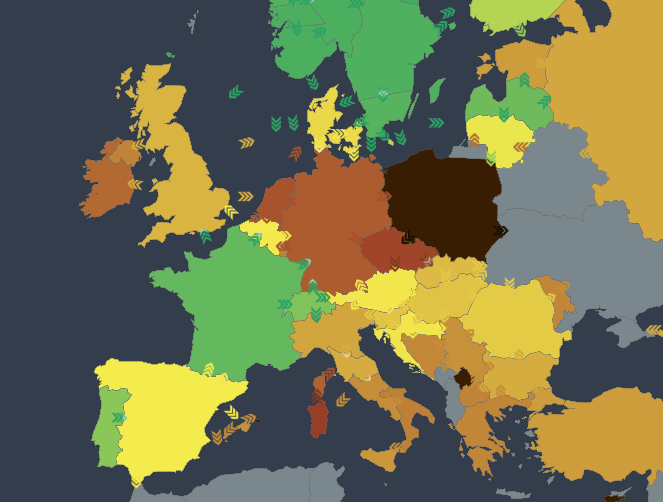
Electricity Maps screen capture focussing on western Europe at 5am.
Mean Carbon Intensity (gCO2eq/kWh) and Power Consumption Breakdown (%) for the year 2023.
# Load libraries library(tidyverse)library(gt)library(showtext)showtext_opts(dpi =300)showtext_auto(enable =TRUE)# Fontsfont_add_google("Fira Sans Condensed")font_add_google("Oswald", "oswald")# Read in datapower_cie_prepared_tbl <-read_csv("data/power_cie_prepared_tbl.csv")# Create table# Note: While the carbon intensity data are freely available, the consumption# (Hydro to Battery Discharge columns) data requires subscription and hence I’ve# created a summary table instead of showing the preceding data wrangling steps.ciep_gt_tbl <- power_cie_prepared_tbl %>%gt() %>%# Apply wider colour range to Carbon Intensity column to mimic source website# colouring: data_color(columns =`CO2 Intensity`,palette =c("#00A600", "#E6E600", "#E8C32E", "#D69C4E" ,"#Dc863B", "sienna", "sienna4","tomato4", "brown"),domain =c(0, 900) ) %>%# Apply colour range to highlight contribution of low-carbon generation to# lower CO2 Intensitydata_color(columns = Hydro:Geothermal,palette =c("#00A600", "chartreuse3", "chartreuse4", "snow") %>%rev(),domain =c(0, 1),apply_to ="fill" ) %>%# Apply colour range to highlight Biomass generation to mid CO2 Intensitydata_color(columns = Biomass,palette =c("snow", "#EEC900", "#E8C32E", "#D69C4E"), #E6E600domain =c(0, 0.3),apply_to ="fill" ) %>%# Apply colour range to highlight fossil fuel contribution to higher CO2 Intensitydata_color(columns = Gas:Oil,palette =c("tomato4", "sienna4", "#D69C4E", "#Dc863B", "snow") %>%rev(),domain =c(0, 1),apply_to ="fill" ) %>%# Assign consistent background colour to remaining columnsdata_color(columns = Unknown:`Battery Discharge`,palette =c("snow") %>%rev(),domain =c(0, 1),apply_to ="fill" ) %>%# Assign the same background to the Zone columndata_color(columns = Zone,palette ="snow",apply_to ="fill" ) %>%# Add header, source note and some styling optionstab_source_note(md("**Table**: @GrantChalmers | **Source**: api.electricitymap.org | **Methodology**: https://www.electricitymaps.com/methodology. Emission factors used to calculate Carbon Intensity can be found on the *Carbon intensity and emission factors* tab.") ) %>%tab_source_note(source_note =md("Some emissions factors are based on IPCC 2014 defaults, while some are based on more accurate regional factors. All zones are publicly available on the *Carbon intensity and emission factors* tab via Google docs [link](https://docs.google.com/spreadsheets/d/1ukTAD_oQKZfq-FgLpbLo_bGOv-UPTaoM_WS316xlDcE/edit?usp=sharing)") ) %>%tab_header(md(str_glue("2023 Mean **Carbon Intensity** (gCO2eq/kWh) and **Power Consumption** Breakdown (%)"))) %>%tab_options(data_row.padding =px(1),table.font.names ="Fira Sans Condensed", #Fira Sans Condensedtable.font.size =12,table.background.color ='snow',heading.background.color ='antiquewhite',column_labels.background.color ='antiquewhite',source_notes.background.color ='antiquewhite',source_notes.font.size =8 ) %>%tab_style_body(style =cell_text(color ="grey60"),values =0 ) %>%tab_style(style =cell_text(color ="#A9A9A9",font ="oswald",size ="xx-small",style ="normal" ),locations =cells_source_notes() ) %>%cols_width(2:last_col() ~px(58) ) %>%cols_align(align ="center",columns =`CO2 Intensity` ) %>%# Convert to percentagefmt_percent(columns = Hydro:`Battery Discharge`,decimals =1,drop_trailing_zeros =TRUE ) %>%fmt_number(columns =`CO2 Intensity`,decimals =0,drop_trailing_zeros =TRUE ) %>%# align decimal points for easier readingcols_align_decimal(# Exclude CO2 Intensitycolumns =3:last_col() ) %>%# Add border to improve aestheticopt_table_outline()# Render tableciep_gt_tbl
2023 Mean Carbon Intensity (gCO2eq/kWh) and Power Consumption Breakdown (%)
Zone
CO2 Intensity
Hydro
Nuclear
Wind
Solar
Geothermal
Biomass
Gas
Coal
Oil
Unknown
Hydro Discharge
Battery Discharge
Sweden
26
39.1%
26.8%
27.7%
0.1%
0 %
0.4%
0.4%
0.8%
0 %
4.6%
0.1%
0 %
Iceland
28
69.4%
0 %
0 %
0 %
30.6%
0 %
0 %
0 %
0 %
0 %
0 %
0 %
Quebec
35
90.1%
2.1%
4.4%
0 %
0 %
1.9%
1.4%
0 %
0 %
0 %
0 %
0 %
France
46
12.3%
65.4%
10.3%
1.8%
0 %
1 %
7.1%
0.3%
0.3%
0.1%
1.4%
0 %
Ontario
104
23.3%
49.4%
8.7%
0.1%
0 %
0.2%
18.1%
0 %
0 %
0 %
0 %
0 %
New Zealand
106
60.5%
0 %
7.7%
0.1%
19 %
0 %
6.8%
3.7%
0 %
2.2%
0 %
0 %
Finland
107
20.2%
36.5%
24.1%
0.1%
0 %
6.2%
3 %
8.1%
0 %
1.8%
0 %
0 %
South Australia
132
0.7%
0 %
42.6%
33.7%
0 %
0 %
13.3%
9 %
0 %
0 %
0 %
0.7%
Spain
132
17.1%
24.2%
25.1%
8 %
0 %
2 %
18.8%
1.3%
0.2%
0.3%
3 %
0 %
Belgium
147
1.3%
39.6%
25.2%
3.6%
0 %
2.8%
19.4%
1.7%
0.1%
4.9%
1.2%
0 %
Tasmania
162
49 %
0 %
22.6%
10.8%
0 %
0 %
1.5%
16.1%
0 %
0 %
0 %
0 %
East Denmark
184
6.4%
5.5%
48.4%
1.3%
0 %
16.8%
7.7%
10.8%
1.4%
1.4%
0.4%
0 %
West Denmark
188
8.8%
2.2%
56.3%
1.6%
0 %
7.6%
8.5%
13 %
0.9%
0.4%
0.6%
0 %
Great Britain
214
3.8%
12.4%
35.9%
2.7%
0 %
6.2%
35.1%
2 %
0 %
1 %
1 %
0 %
Netherlands
218
1.1%
3.9%
46.7%
10.8%
0 %
4.6%
22.4%
8.6%
0.8%
1.1%
0.2%
0 %
New York ISO
275
23.7%
22.8%
4.9%
0 %
0 %
0.1%
46.9%
0 %
0 %
1.6%
0 %
0 %
Italy (North)
307
22.7%
14.5%
3.9%
2.9%
0.2%
3.1%
38.4%
1.5%
0.2%
9.3%
3.3%
0 %
California
328
8.4%
12.7%
7.9%
12 %
3 %
1.8%
48.5%
2.1%
0 %
1.2%
0 %
2.6%
Germany
389
4.4%
2.8%
39.7%
3.3%
0 %
8.7%
14.4%
23.3%
0.6%
0.6%
2.1%
0 %
Ireland
389
3.7%
0.8%
38.5%
0.2%
0 %
2.5%
42.4%
9.7%
2 %
0.1%
0.1%
0 %
Western Australia
417
0 %
0 %
14.1%
33.8%
0 %
0.3%
24.2%
27.1%
0.3%
0 %
0 %
0.3%
Texas
432
0 %
9.1%
22.3%
6 %
0 %
0 %
46.1%
16.1%
0 %
0.4%
0 %
0 %
Alberta
447
1.9%
0 %
12.4%
1.1%
0 %
2.5%
70.7%
7.2%
0 %
4.1%
0 %
0 %
Victoria
508
3.9%
0 %
17.5%
19 %
0 %
0 %
0.3%
59.1%
0 %
0 %
0 %
0.2%
New South Wales
578
3.2%
0 %
9.5%
23.7%
0 %
0.2%
0.7%
62.6%
0 %
0 %
0 %
0.1%
Queensland
662
1.9%
0 %
3.8%
21.1%
0 %
0 %
7.2%
65.7%
0.2%
0 %
0 %
0.1%
South Africa
685
2.2%
4.3%
5.8%
3.8%
0 %
0 %
0 %
79.9%
2 %
0.1%
2 %
0 %
India (North)
693
9.3%
2.2%
0.1%
10.6%
0 %
0 %
1.8%
75.2%
0 %
0.9%
0 %
0 %
Table: @GrantChalmers | Source: api.electricitymap.org | Methodology: https://www.electricitymaps.com/methodology. Emission factors used to calculate Carbon Intensity can be found on the Carbon intensity and emission factors tab.
Some emissions factors are based on IPCC 2014 defaults, while some are based on more accurate regional factors. All zones are publicly available on the Carbon intensity and emission factors tab via Google docs link